What is the formula for drop down list in Excel?

Dependent drop-down lists offer straightforward and scalable solutions to several Excel challenges.

The subscription version of Excel offers an easy way to create dependent drop-down lists. A drop-down list is an input interface that lists options to choose from. This reduces the amount of typing and errors.

A dependent drop-down is one that populates its list based on a previous drop-down selection. Unlike in previous versions of Excel, this solution is straightforward and scalable.

We will use the table in Figure 1 as the basis for three separate drop-down selections. (Note: Gadgets dont have an extra-large size, and the colours vary between sizes.)

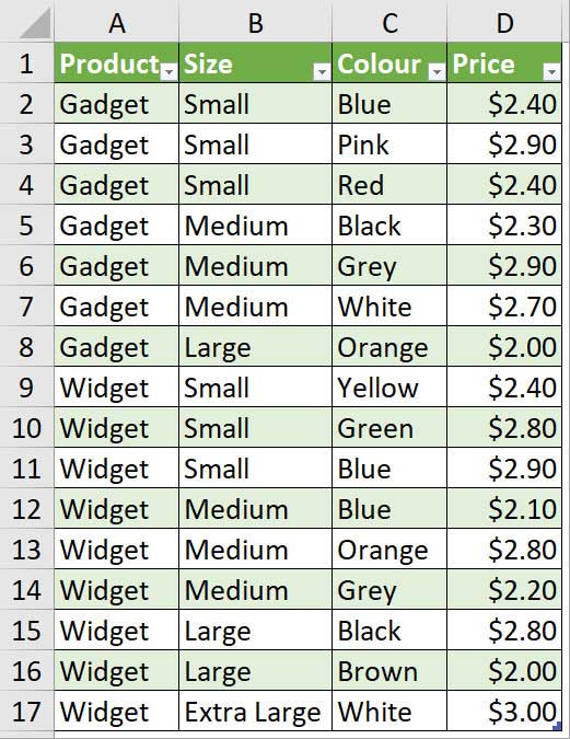
The table in Figure 1 is a formatted table. This means the table range automatically expands as data is added to the table, and our solution will also be scalable and will adjust as new products are added to the table.

We will create the drop-down list in the yellow cells in Figure 2, using the section on the right.

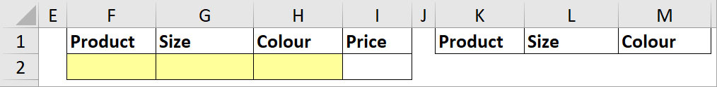
We will create the list for the cell F2 drop-down in column K.

The formula for cell K2 is:

=UNIQUE(tblProd[Product])

tblProd is the name I have given the formatted table. Square brackets are used to define a column in the table.

Figure 3 shows how the formula in cell K2 spills down (expands) to include the two products.

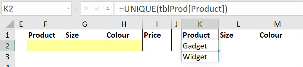
This is part of the dynamic array feature included in the subscription version of Excel.

Creating a drop-down

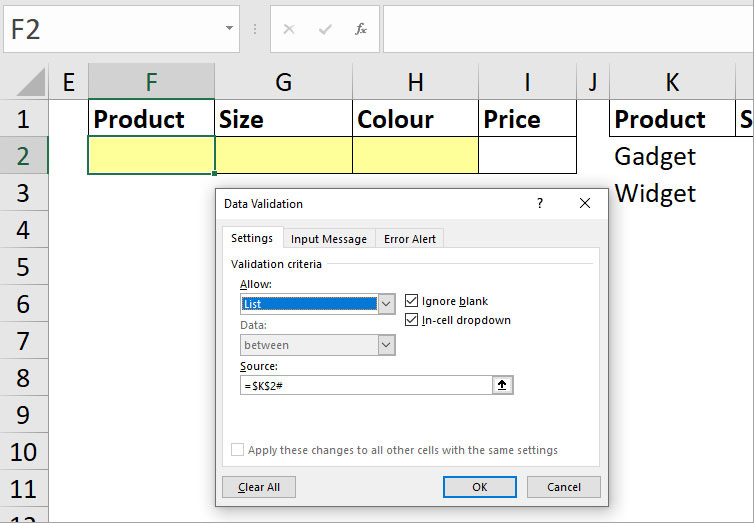
To create the drop-down for cell F2, we can use a keyboard shortcut to open the Data Validation dialog. Press Alt A V V in sequence, without holding down the keys.

In the dialog that opens, select List from the Allow drop-down. Click in the Source box and use the mouse to click on cell K2, then type # (see Figure 4). Adding the # symbol to the end refers to the spill range that starts in cell K2.

This new symbol is part of the dynamic array functionality. Click OK, and the first drop-down is ready.

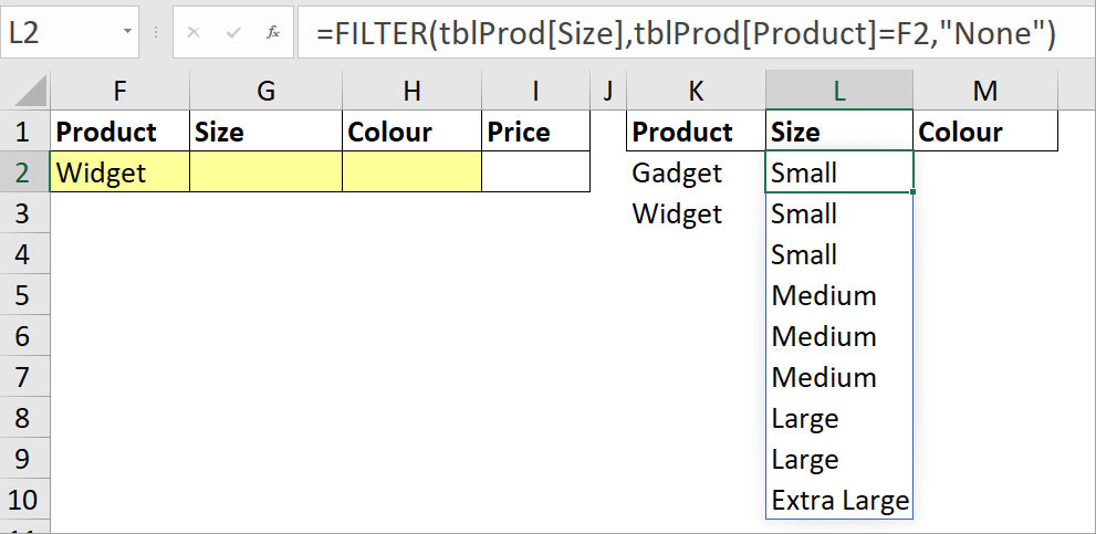
The Size drop-down list (cell G2) is dependent on the Product chosen in cell F2. I will create the list in cell L2 in two steps. The initial formula will use the FILTER function. In cell L2, enter the following formula:

=FILTER(tblProd[Size],tblProd[Product]=F2,None)

This formula lists all the Sizes (including duplicates) related to the product chosen in cell F2 (see Figure 5). The None in the formula specifies what to display if the condition is not met in this case, if cell F2 is empty.

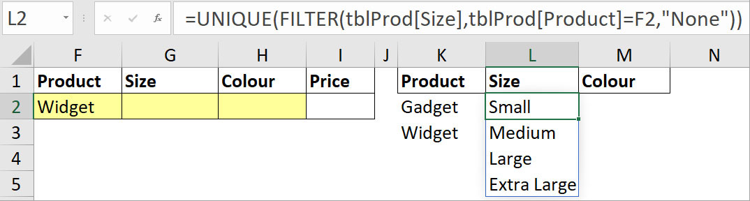
This list is not suitable for a drop-down list, as the entries are duplicated. We can wrap the UNIQUE function around the FILTER function to remove duplicates. The final formula for cell L2 is:

=UNIQUE(FILTER(tblProd[Size],tblProd[Product]=F2,None))

Figure 6 shows the result.

We can now create the drop-down for cell G2. Press Alt A V V. Use the List in the Allow drop-down, click in the Source box, click cell L2, add the # and click OK.

The list for the cell H2 drop-down is more complex, because we need to use two conditions in the FILTER function. The formula for cell M2 is:

=FILTER(tblProd[Colour],(tblProd

[Product]=F2)*(tblProd[Size]=G2),None)

How to handle two conditions

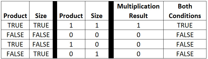
To handle two conditions, we enclose each condition within brackets and multiply them together. In Excel, TRUE = 1 and FALSE = 0. When you multiply the results together, they are converted to their respective values. This creates a single result for each row, either 1 or 0.

Excel will treat 1 as TRUE and 0 as FALSE to determine which rows to display. The table in Figure 7 shows the four possible results when analysing two conditions.

We dont need to use the UNIQUE function in cell M2, as the entries are already unique. You can, however, sort the list using the new SORT function. The revised formula is:

=SORT(FILTER(tblProd[Colour],(tblProd

[Product]=F2)*(tblProd[Size]=G2),None))

We can now create the drop-down for cell H2. Press Alt A V V, use the List in the Allow drop-down, click in the Source box, click cell M2, add the # and click OK.

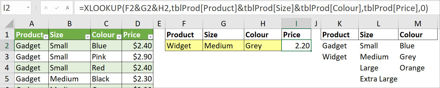
Now that we have three separate selections, we can return the price for that combination from the table.

In the subscription version we can perform some magic with the XLOOKUP function and perform a lookup based on three entries.

The formula for cell I2 is:

=XLOOKUP(F2&G2&H2,tblProd

[Product]&tblProd[Size]&tblProd

[Colour],tblProd[Price],0)

We use & to join the three entries together. We then use & to join the three columns in the table to create a combined list to look up. The Price column is returned based on the combined entries being found. If the entry is not found, zero is returned.

Figure 8 shows the final structure.

The new dynamic array functions and features work well together and offer many new ways to solve problems in Excel. The companion video to this article demonstrates the scalability of this solution.

The companion video and Excel files (blank and complete) will go into more detail to demonstrate these techniques.

Neale Blackwood CPA runs A4 Accounting, providing Excel training, webinars and consulting services. Questions can be sent to [emailprotected]